Monty Hall problem: Understanding & Visualization

Last updated on Mar 10, 2022 13 min read Blog

Problem Description

Monty Hall Problem is one of the most popular probability puzzles. The problem describes a game show where the participant has to choose among three doors, only one of which contains a prize behind it.

The rules of the game are as the following.

You first choose a door and let the host know. (Original Choice, ▦).
The host knows which door has the prize, and opens one of the the (un-chosen) doors which doesn’t have the prize behind it. This door is then eliminated. (Eliminated Choice, ◽).
You now have the option of sticking with your Original Choice, or changing to the other remaining door after elimination (Alternate Choice, ▦).

The question is whether you are better off sticking to your Original Choice, or switching to the Alternate Choice after the elimination, or if it doesn’t matter. Apparently, majority of the people think that it doesn’t matter whether you stick to your original choice or change your choice to the remaining door, as both of them are expected to have 33% chance of success originally. But, it is now well known that the chances of success are better if we switch to the remaining door after elimination.

In this post, I will try to look at the Monty Hall problem in 3 different ways, in an unnecessary amount of detail 😄, unless, of course, you are one of the kind who would get inspired by 120 different proofs of Pythagoras theorem (link). The code for this post and visualizations can be found here.

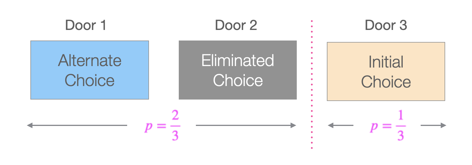
Approach 1 - A Thought Experiment

Let us assume we choose Door 3 initially.
Let us also imagine Door 1 + Door 2 as one unit, and Door 3 as the second unit as shown below.
- We can see that the probability of success for the Door 1 + Door 2 unit is \(\frac{2}{3}\).
Now, imagine if the host gives us the ability to choose that entire unit (consisting of two doors) instead of Door 3. We would obviously choose that unit, as it has a \(\frac{2}{3}\) probability of success.
When the host eliminates Door 2 and gives us an option to choose Door 1 (or vice versa), he is effectively giving us the option to choose the entire unit of Door 1 + Door 2. So, when we leave our original choice (Door 3) behind, and switch to the other non-eliminated door in the two door unit, we have a higher probability of success \(\frac{2}{3}\).

While the above explanation may be intuitive enough for some people, it may still appear a little hand-waving. So, we will explore a couple more approaches below.

Approach 2 - Simulations

We can verify if logic from the above argument is true, by simulating this experiment a large number of times. In this section, we simulate the experiment 30 times, and use the visuals below to understand the results.

set.seed(2017)

# number of runs
n <- 30

# make a data frame containing three columns called door1, door2, door3.
# Each row should contain two "goat"s and one "car", randomly distributed
# among three columns

car_positions <- sample(1:3, n, replace = TRUE)

# run the experiment chosen number of times
df_experiment_runs <-
  ldply(car_positions, function(x)
    ifelse(1:3 == x, "car", "goat"))
names(df_experiment_runs) <- c("Door1", "Door2", "Door3")
df_experiment_runs$`Run Number` <-
  as.numeric(row.names(df_experiment_runs))
df_experiment_runs$`First Choice` <- sample(1:3, n, replace = TRUE)
df_experiment_runs$`Prize Location` <- car_positions
df_experiment_runs$`Eliminated Position` <- apply(
  df_experiment_runs,
  MARGIN = 1,
  FUN = function(x) {
    (
      setdiff(1:3, c(x['Prize Location'], x['First Choice']))
        [sample(length(setdiff(1:3, c(x['Prize Location'], x['First Choice']))), 1)]
    )
  }
)

df_experiment_runs$`Alternate Choice` <- apply(
  df_experiment_runs,
  MARGIN = 1,
  FUN = function(x) {
    (
      setdiff(1:3, c(x['Eliminated Position'], x['First Choice']))
        [sample(length(setdiff(1:3, c(x['Eliminated Position'], x['First Choice']))), 1)]  
    )
    
  }
  
)


df_experiment_runs$Winning_Choice <-ifelse(
  df_experiment_runs$`Prize Location` == df_experiment_runs$`Alternate Choice`,
  "Alternate Choice",
  "Original Choice"
)

df_experiment_runs <- df_experiment_runs %>%
  group_by(Winning_Choice) %>% mutate(y2 = row_number())


df_experiment_runs_long <- pivot_longer(df_experiment_runs,
                                        cols = starts_with("Door"),
                                        names_to = "Door")
df_experiment_runs_long$Door <-
  gsub('Door', '', df_experiment_runs_long$Door)

df_experiment_runs_long$Door_modified <-
  as.integer(df_experiment_runs_long$Door) + as.integer(
    df_experiment_runs_long$`Prize Location` == df_experiment_runs_long$`Alternate Choice`
  ) * 4

df_legend <-
  expand_grid(
    Choices = c(
      "Prize\nLocation",
      "Original\nChoice",
      "Winning\nOriginal Choice",
      "Eliminated\nChoice",
      "Winning\nAlternate Choice"
    )
  )
df_legend$Choices <- fct_inorder(df_legend$Choices)

# Generate a plot to be used for the legend.
get_legend_plot <- function(df) {
  ggplot(df, aes(x = Choices, fill = Choices, y = 1)) +
    geom_tile(color = 'gray50',
              width = 0.13,
              height = 1) +
    coord_cartesian(ylim = c(0, 2)) +
    facet_grid(~ Choices, scales = 'free') +
    geom_point(data = df %>% filter(grepl("Prize|Winning", Choices)), size = 1) +
    scale_fill_manual(values = c("Prize\nLocation" = 'white', "Original\nChoice" = 'bisque', "Eliminated\nChoice" = 'gray70', "Winning\nOriginal Choice" = 'bisque', "Winning\nAlternate Choice" = 'lightskyblue')) +
    theme_void() +
    
    theme(
      legend.position = 'none',
      axis.text.x = element_text(size = 9),
      strip.text = element_blank()
    )
}

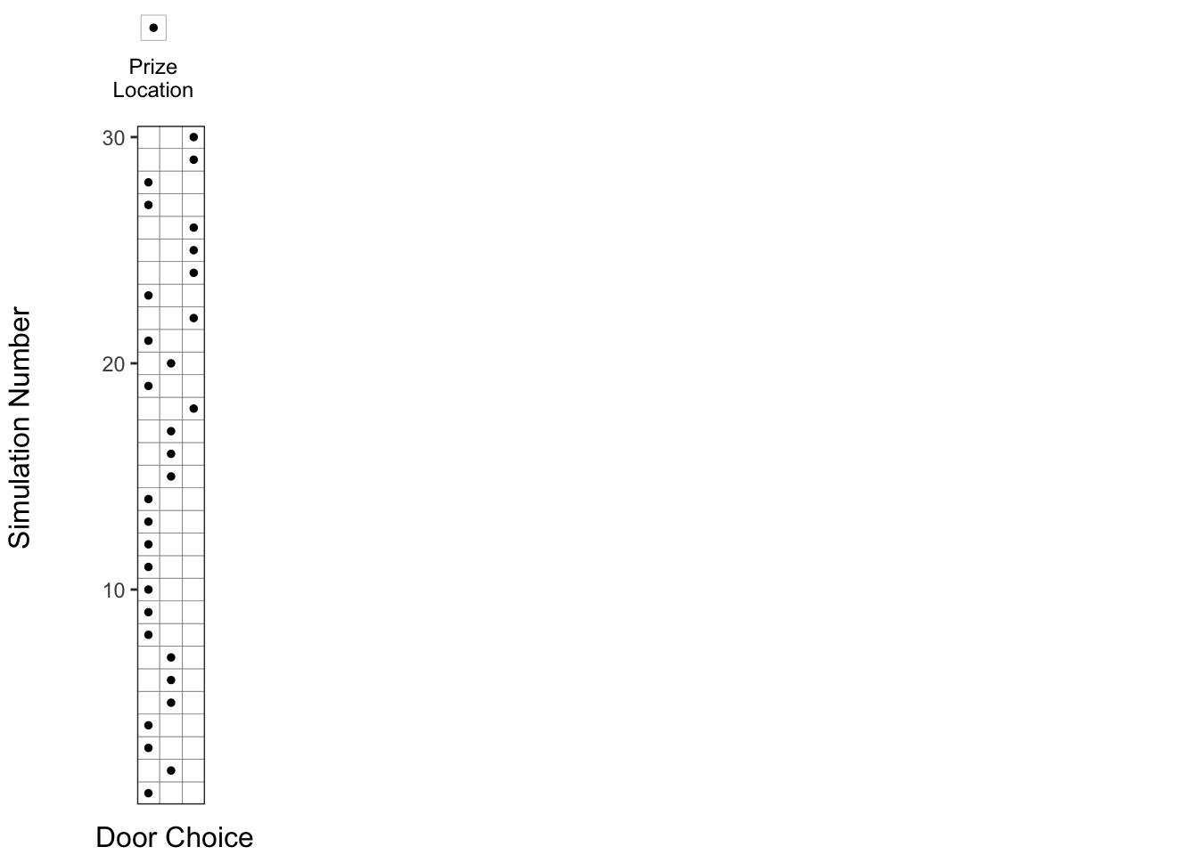
1. Prize locations chosen at random:

First, let us denote the Prize Locations in each of the 30 runs by a dot (.), which is chosen randomly among the 3 doors.

get_permutation_grid <- function(df){
  df_all_combinations <- expand.grid(`Run Number` = (1:nrow(df)), Door = (1:3)) 
  
  ggplot(df_all_combinations, aes(y = `Run Number`, x = Door)) +
  geom_tile(fill = 'white', color = 'gray40') +
  scale_y_continuous(expand = expansion(0, 0)) +
  scale_x_discrete(expand = expansion(0, 0)) +
  coord_equal() +
  theme_bw() +
  theme(
    legend.position = 'none',
    axis.title = element_blank(),
    plot.subtitle = element_text(hjust = 0.5)
  )
}

p0 <- get_permutation_grid(df_experiment_runs)


p1 <-
  p0 + geom_point(data = df_experiment_runs, aes(x = `Prize Location`), size = 1) +
  # labs(subtitle = 'Prize Locations') +
  NULL

annotate_figure(
  ggarrange(
    ggarrange(
      get_legend_plot(head(df_legend, 1)),
      NULL,
      NULL,
      NULL,
      NULL,
      nrow = 1,
      align = 'h'
    ),
    NULL,
    ggarrange(p1, NULL, NULL, NULL, NULL, nrow = 1, align = 'h'),
    nrow = 3,
    heights = c(1.4, 0.2, 10)
  ),
  #
  #     ncol = 2, align = 'h'
  left = text_grob("Simulation Number", rot = 90, size = 12),
  bottom = text_grob(
    "Door Choice",
    size = 12,
    hjust = 0,
    x = 0.05
  )
)

2. Original door choice chosen at random:

Then, let us show the original choice of the doors, denoted by an orange square (▦), which are also chosen at random.

p2 <-
  p0 + geom_tile(
    data = df_experiment_runs,
    aes(x = `First Choice`),
    fill = 'bisque',
    color = 'gray40'
  ) 
annotate_figure(
  ggarrange(
    ggarrange(
      get_legend_plot(head(df_legend, 2)),
      NULL,
      widths = c(0.4, 0.6),
      nrow = 1,
      align = 'h'
    ),
    NULL,
    ggarrange(p1, p2, NULL, NULL, NULL, nrow = 1, align = 'h'),
    nrow = 3,
    heights = c(1.4, 0.2, 10)
  ),
  left = text_grob("Simulation Number", rot = 90, size = 12),
  bottom = text_grob(
    "Door Choice",
    size = 12,
    hjust = 0,
    x = 0.15
  )
)

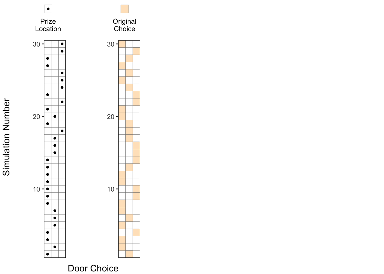
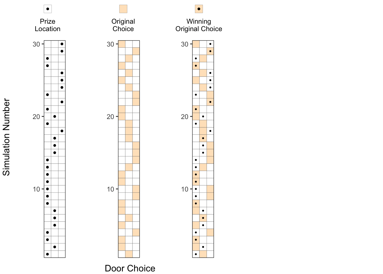
3. Original choice combined with prize locations:

When we combine the above two plots, we can see how many times we choose the door containing a prize indicated by an orange square with a dot in the picture below.

No. of successes with original choice = No. of orange squares with a dot

In the plot below, we can say about 10 out of 30 trials result in a success where the prize location, is same as the original choice, as expected, with about probability.

p3 <-
  p2 + geom_point(data = df_experiment_runs, aes(x = `Prize Location`), size = 0.5)

annotate_figure(
  ggarrange(
    ggarrange(
      get_legend_plot(df_legend[c(1,2,3),]),
      NULL,
      widths = c(0.6, 0.4),
      nrow = 1,
      align = 'h'
    ),
    NULL,
    ggarrange(p1, p2, p3, NULL, NULL, nrow = 1, align = 'h'),
    nrow = 3,
    heights = c(1.4, 0.2, 10)
  ),
  left = text_grob("Simulation Number", rot = 90, size = 12),
  bottom = text_grob(
    "Door Choice",
    size = 12,
    hjust = 0,
    x = 0.25
  )
)

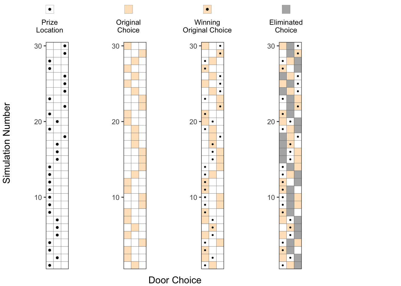
4. Eliminating one of the doors without the prize:

At this point, the host would eliminate one of the doors which doesn’t contain the prize and is not chosen as the original choice. We denote this eliminated choice by a gray square (◽). You can see that for some of the experiments, the host can choose one of the two doors to eliminate (eg. runs 3, 11 and 12), but in some other experiments, he has only one choice to eliminate (eg. runs 1, 2, 4).

p4 <-
  p3 + geom_tile(
    data = df_experiment_runs,
    aes(x = `Eliminated Position`),
    fill = 'gray70',
    color = 'gray40'
  )

annotate_figure(
  ggarrange(
    ggarrange(
      get_legend_plot(head(df_legend, 4)),
      NULL,
      widths = c(0.8, 0.2),
      nrow = 1,
      align = 'h'
    ),
    NULL,
    ggarrange(p1, p2, p3, p4, NULL, nrow = 1, align = 'h'),
    nrow = 3,
    heights = c(1.4, 0.2, 10)
  ),
  left = text_grob("Simulation Number", rot = 90, size = 12),
  bottom = text_grob(
    "Door Choice",
    size = 12,
    hjust = 0,
    x = 0.35
  )
)

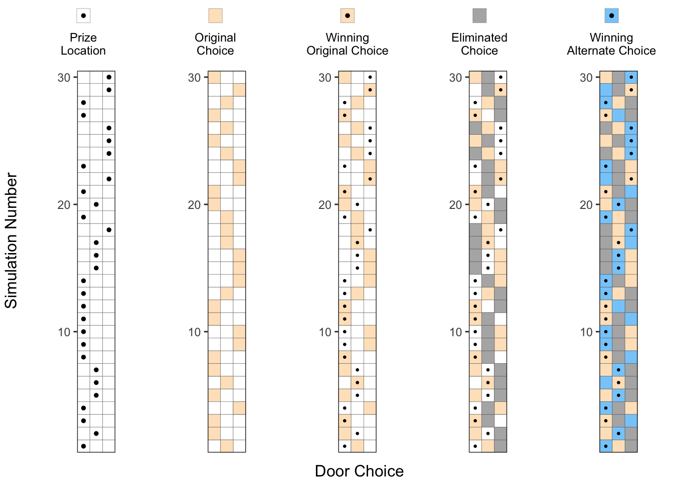
5. Considering the alternate choice:

After one of the doors is eliminated, we have the option of changing our choice to the alternate door, which is denoted by a blue square (▦) in this picture.

No. of successes with alternate choice = No. of blue squares with a dot

If we count carefully, we can see that there about 20 blue squares with a dot in this experiment of 30 runs, which is about twice the probability of success compared to the original choice.

get_p5 <- function(df_experiment_runs, y_var = "Run Number"){
  p0_tmp <- get_permutation_grid(df_experiment_runs)
  p5_tmp <- p0_tmp + 
    geom_tile(
      data = df_experiment_runs,
      aes(x = `Eliminated Position`, y = get(y_var)),
      fill = 'gray70',
      color = 'gray40'
  ) +
  geom_tile(
    data = df_experiment_runs,
    aes(x = `First Choice`, y = get(y_var)),
    fill = 'bisque',
    color = 'gray40'
  ) +
  geom_tile(
    data = df_experiment_runs,
    aes(x = `Alternate Choice`, y = get(y_var)),
    fill = 'lightskyblue',
    color = 'gray40'
  ) +
  geom_point(
    data = df_experiment_runs,
    aes(x = `Prize Location`, y = get(y_var)), 
    size = 0.5) + 
  scale_y_continuous(limits = c(0.5,30.5), expand = expansion(0,0)) + 
  theme(panel.grid.major = element_blank(),
        panel.grid.minor = element_blank())
  return(p5_tmp)
}

p5 <- get_p5(df_experiment_runs)

annotate_figure(
  # ggarrange(p1, p2, p3, p4, p5, nrow = 1, align = 'h'),
  ggarrange(
    get_legend_plot(head(df_legend, 5)),
    NULL,
    ggarrange(p1, p2, p3, p4, p5, nrow = 1, align = 'h'),
    nrow = 3,
    heights = c(1.4, 0.2, 10)
  ),
  left = text_grob("Simulation Number", rot = 90, size = 12),
  bottom = text_grob(
    "Door Choice",
    size = 12,
    hjust = 0,
    x = 0.45
  )
)

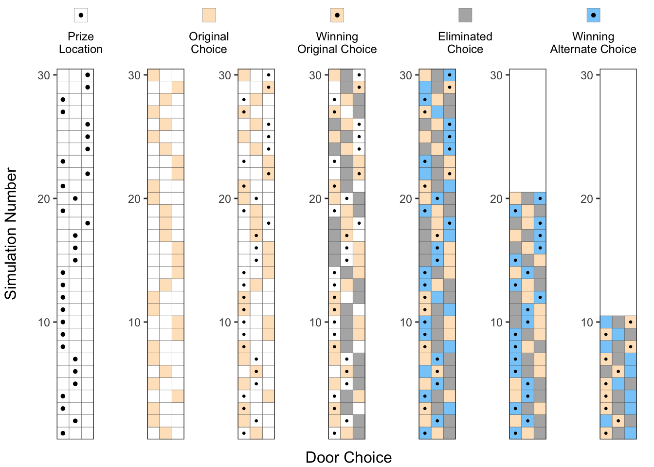
Just to make it clearer, we can separate the simulations where the Alternate Choice (▦) was the winning choice, and where the Original Choice (▦) was the winning choice, as shown in the two right-most plots below. Now, we can clearly see that changing our choice after the elimination of one of the doors, improved the success probability by about 2x.

p5_a <- get_p5(df_experiment_runs %>% filter(Winning_Choice == "Alternate Choice"), y_var = "y2")
p5_b <- get_p5(df_experiment_runs %>% filter(Winning_Choice == "Original Choice"), y_var = "y2")

annotate_figure(
  # ggarrange(p1, p2, p3, p4, p5, nrow = 1, align = 'h'),
  ggarrange(
    get_legend_plot(head(df_legend, 5)),
    NULL,
    ggarrange(p1, p2, p3, p4, p5, p5_a, p5_b, align = 'v', nrow = 1),
    nrow = 3,
    heights = c(1.4, 0.2, 10)
  ),
  left = text_grob("Simulation Number", rot = 90, size = 12),
  bottom = text_grob(
    "Door Choice",
    size = 12,
    hjust = 0,
    x = 0.45
  )
)

Approach 3 - Exact Probability Calculations

Though the previous simulations make sense, they do not provide a definitive proof that switching our door choice would increase our probability of success to 2/3. As a matter of fact, there could be a different set of 30 simulation runs where the results could be the opposite of what we got (though less likely). So, in this section we try to provide a more rigorous permutations-based calculations to get these probabilities.

First, the host 3 doors to choose from for placing the prize, and we have 3 doors to choose from for our initial choice. As shown below, we have total 9 possible permutations, each having an equal probability of 9.

permutation_data <- expand.grid(
  `Prize Location` = (1:3),
  `First Choice` = (1:3),
  `Eliminated Position` = (1:3)
) %>% filter((`Eliminated Position` != `Prize Location`) &
               (`Eliminated Position` != `First Choice`)) %>% 
  arrange(`Prize Location`, `First Choice`)

get_unique_permutations <- function(df, column_list) {
  df_permutations <-
    df %>% distinct(across(all_of(column_list)))
  df_permutations$`Run Number` <- seq(nrow(df_permutations))
  return(df_permutations)
}

df_pre_elimination <- get_unique_permutations(permutation_data, c("Prize Location", "First Choice"))

p0 <- get_permutation_grid(df_pre_elimination) + scale_y_continuous(breaks = (1:9), expand = expansion(0,0))

p1 <-
  p0 + geom_point(data = df_pre_elimination, aes(x = `Prize Location`), size = 2) +
  NULL

p2 <-
  p0 + geom_tile(
    data = df_pre_elimination,
    aes(x = `First Choice`),
    fill = 'bisque',
    color = 'gray40'
  ) 

p3 <- p2 + 
  geom_point(data = df_pre_elimination, aes(x = `Prize Location`), size = 2) #+ annotate("text", x = 3.8, y = (1:9), label = "1/9", size = 3)

p_123 <- annotate_figure(
  ggarrange(
    ggarrange(
      get_legend_plot(df_legend[c(1,2,3),]),
      NULL,
      widths = c(0.6, 0.4),
      nrow = 1,
      align = 'h'
    ),
    ggarrange(p1, p2, p3, NULL, NULL, nrow = 1, align = 'h'),
    nrow = 3,
    heights = c(1.3, 9)
  ),
  left = text_grob("Permutation", rot = 90, size = 12),
  bottom = text_grob(
    "Door Choice",
    size = 12,
    hjust = 0,
    vjust = -4,
    x = 0.25
  ),
  right = text_grob(paste(rep("p = 1/9",9), collapse="\n") , hjust = 5.2, lineheight = 1.55, vjust = 0.45)
)
p_123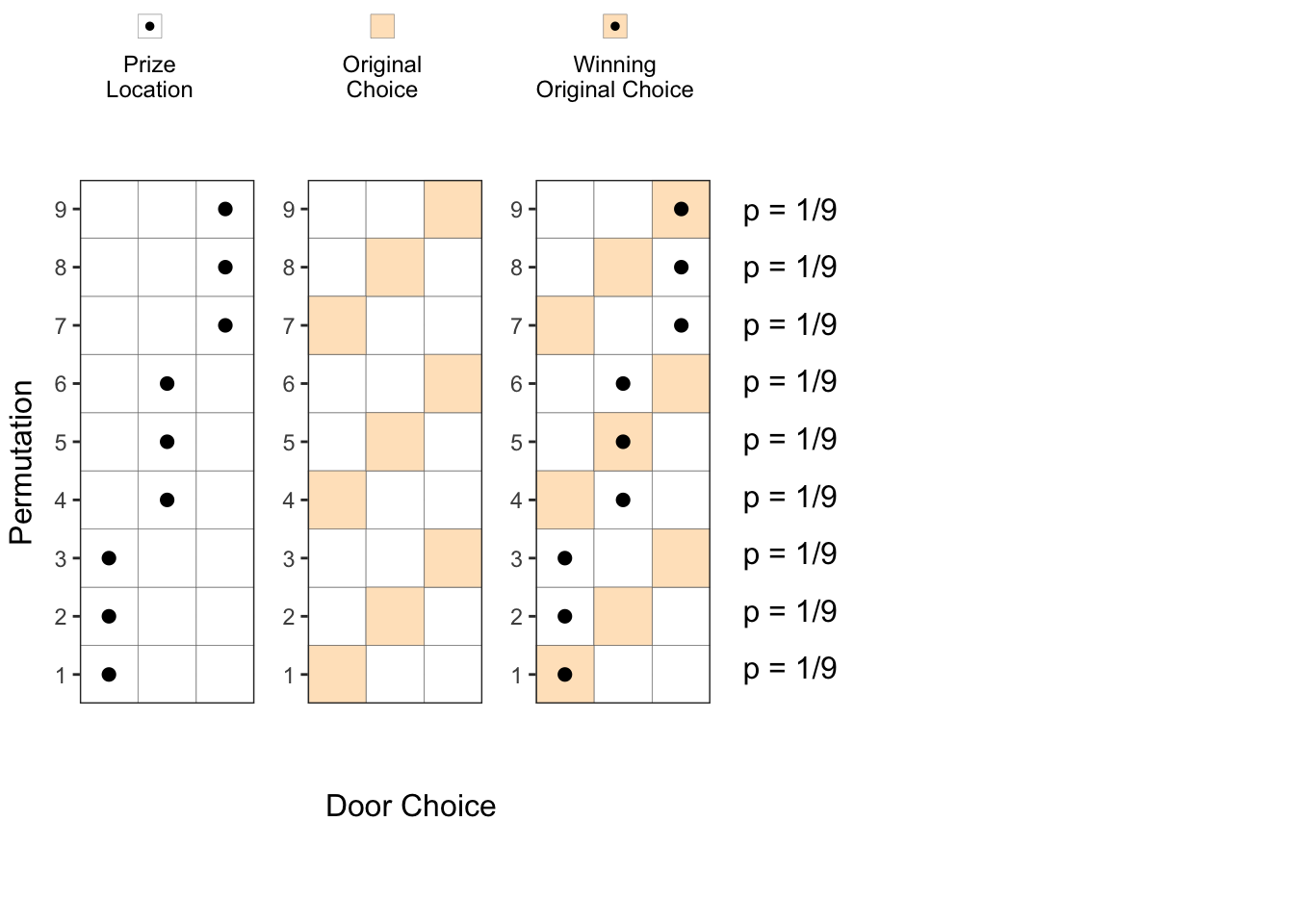

Next step is for the host to eliminate one of the two un-chosen doors. However, he cannot eliminate a door which has a prize. So, some of the permutations above result in two choices for the host to eliminate from, and in the other cases, the host can eliminate only one of the doors.

In permutations 1, 5, and 9, the host has two choices for the door elimination, and hence these can be divided into permutations 1a, 1b, 5a, 5b and 9a, 9b respectively with half the probability each (\(\frac{1}{18}\)) after the elimination step. For the other permutations, the host has only one choice for elimination, so the probability of that permutation remains unchanged at \(\frac{1}{9}\) both before and after elimination, as shown below.

df_post_elimination <- get_unique_permutations(permutation_data, c("Prize Location", "First Choice", "Eliminated Position"))
df_post_elimination$`Alternate Choice` <- apply(
  df_post_elimination,
  MARGIN = 1,
  FUN = function(x) {
    (
      setdiff(1:3, c(x['Eliminated Position'], x['First Choice']))
        [sample(length(setdiff(1:3, c(x['Eliminated Position'], x['First Choice']))), 1)]  
    )
    
  }
  
)
df_post_elimination$probs = "p=1/9"

p4_a <- get_permutation_grid(df_post_elimination) + 
  scale_y_continuous(breaks = (1:12), 
                     labels = c("1a", "1b", "2", "3", 
                                "4", "5a", "5b", "6",
                                "7", "8", "9a", "9b"), 
                     expand = expansion(0,0)) + 
  geom_tile(
    data = df_post_elimination,
    aes(x = `First Choice`),
    fill = 'bisque',
    color = 'gray40'
  )+ 
  geom_tile(
    data = df_post_elimination,
    aes(x = `Eliminated Position`),
    fill = 'gray70',
    color = 'gray40'
  ) + 
  geom_tile(
    data = df_post_elimination,
    aes(x = `Alternate Choice`),
    fill = 'lightskyblue', #'darkolivegreen3', #'bisque',
    color = 'gray40'
  ) + 
  geom_point(data = df_post_elimination, aes(x = `Prize Location`), size = 2) 

p5_a <-  get_permutation_grid(df_post_elimination) + 
  scale_y_continuous(breaks = (1:12), 
                      labels = c("1a", "1b", "2", "3",
                                "4", "5a", "5b", "6",
                                "7", "8", "9a", "9b"),
                     expand = expansion(0,0)) + 
  geom_tile(
    data = df_post_elimination,
    aes(x = `Eliminated Position`),
    fill = 'gray70',
    color = 'gray40'
  ) +
  geom_tile(
    data = df_post_elimination,
    aes(x = `Alternate Choice`),
    fill = 'lightskyblue', #'darkolivegreen3', #'bisque',
    color = 'gray40'
  ) + 
  geom_point(data = df_post_elimination, aes(x = `Prize Location`), size = 2) 


annotate_figure(
  ggarrange(
    get_legend_plot(head(df_legend, 5)),
    NULL,
    ggarrange(ggarrange(p1, p2, p3, align = 'v', nrow = 1),
              NULL,
              ggarrange(p4_a, align = 'v', nrow = 1),
              nrow = 1,
              widths = c(2, 0.3, 1)
              ),
    nrow = 3,
    heights = c(1.4, 0.1, 10)
  ),
  left = text_grob("Permutation", rot = 90, size = 12),
  bottom = text_grob(
    "Door Choice",
    size = 12,
    hjust = 0,
    x = 0.45
  ),
  right = text_grob(paste(c("p = 1/18","p = 1/18", "p = 1/9", "p = 1/9", 
                            "p = 1/9", "p = 1/18","p = 1/18", "p = 1/9",  
                             "p = 1/9", "p = 1/9", "p = 1/18","p = 1/18"
                            ), collapse="\n") , hjust = 0.8, lineheight = 1.7, vjust = 0.55)
)

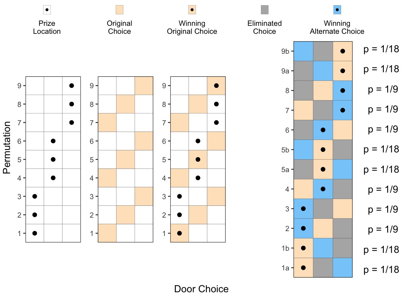
Now, if we add up all the probabilities for Winning Alternative Choices (Blue squares with a dot), we can see that they add up to \(\frac{6}{9} = \frac{2}{3}\). Similarly, if we add all the probabilities for the Winning Original Choices (Orange squares with a dot), we can see that they add up to \(\frac{6}{18} = \frac{1}{3}\). So, we have conclusively proved that changing our choice after the host eliminates one of the doors is the better option.

Conclusion

We have looked at the Monty Hall problem in 3 different ways to arrive at the same answer. I hope this gives you better insight into this problem.

Next Steps

I can’t believe there are still things to explore after spending so much time on this post. However, here are a couple more things that I am planning to investigate when I get a chance.

Trying to arrive at the same answer using a Bayesian approach
Practical implications of the Monty Hall Problem and other similar problems

Visualization Probability R

Seshadri Kolluri

Data Scientist & Hardware Engineer

My research interests include data science, data visualization, machine learning, Gallium Nitride electronics, and semiconductor technology development.